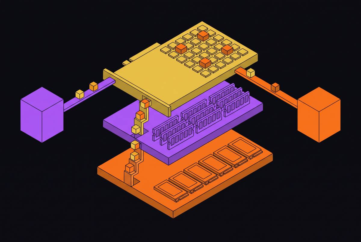
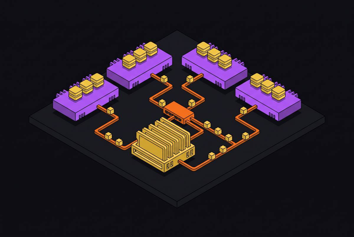
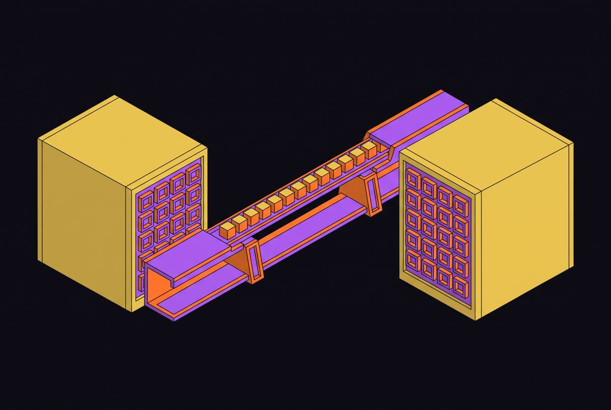
Weight Streaming Architectures That Eliminate GPU Idle Time During Model Loading
Streaming weights concurrently from object storage can reclaim most GPU minutes lost to cold starts.
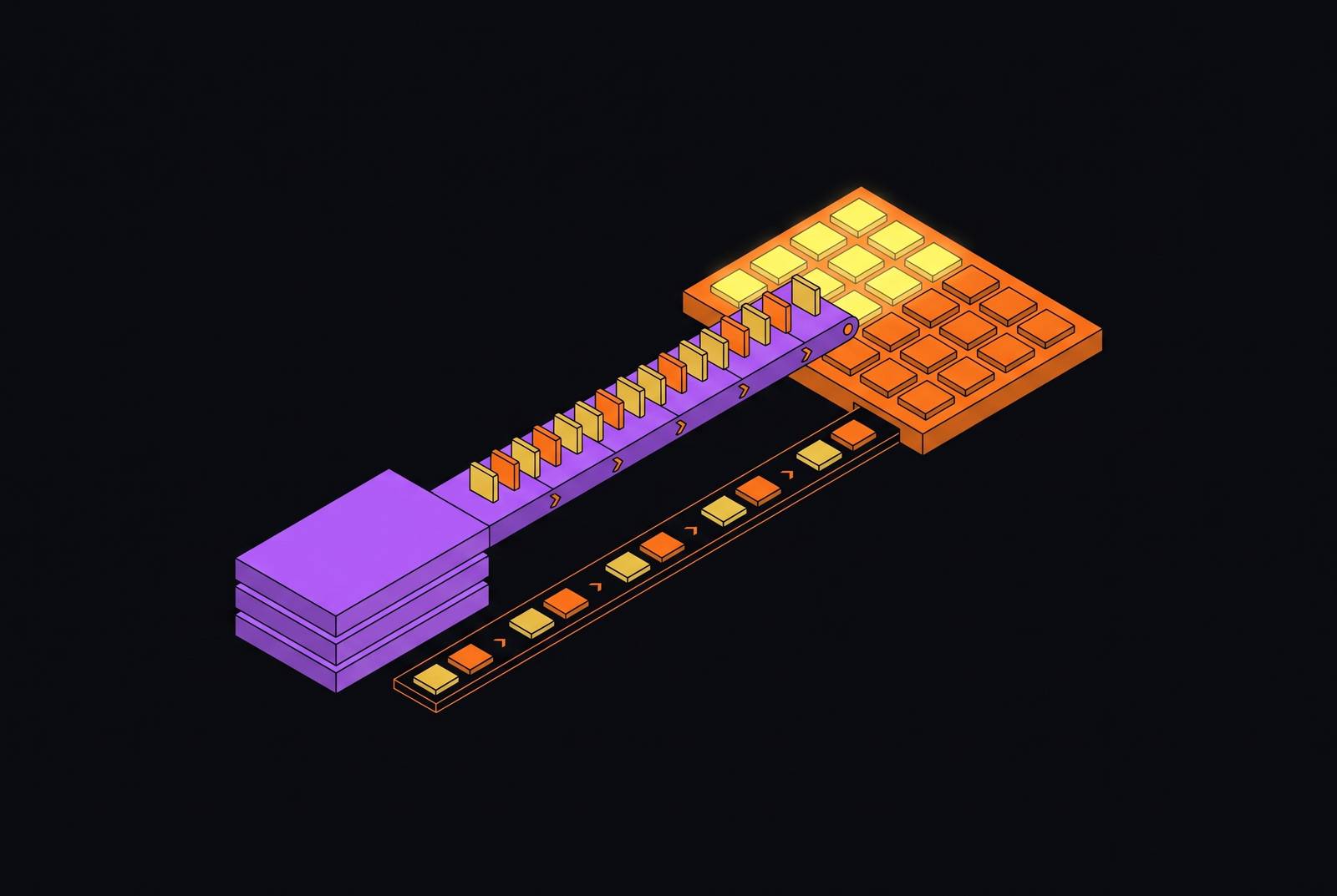
Weight streaming architectures reduce GPU idle time during model loading by replacing sequential download-then-load steps with concurrent reads from object storage and overlapping transfers into GPU memory. The storage architecture determines the gain. For LLM inference throughput, NVMe and tiered storage place frequently used weights and cache data on faster paths, while sustained bandwidth determines how quickly those bytes reach the GPU.
Why GPUs sit idle during model loading and why it costs real money
An allocated GPU consumes power and budget even when model loading leaves it with no useful compute. The Energy Cost of Execution-Idle in GPU Clusters identified this low-activity, power-hungry state across training, inference, and serving workloads on six GPU generations, including NVIDIA B200. Many idle intervals followed I/O bottlenecks. The finding connects wasted energy to storage and memory transfers as well as inefficient algorithms.
Cold starts make that cost recur. Scaling events, restarts, rolling deployments, and model swaps can each trigger another download followed by another load into GPU memory. Even with fast local NVMe, a large model can take tens of seconds to load. During that interval, the new replica consumes allocated capacity but cannot serve requests, while existing replicas absorb the traffic.
The two distinct GPU idle problems and why only one is "weight streaming"
Cold-start idle begins outside the GPU. The default path downloads the full model from object storage to local disk, then copies it into GPU memory. Local disk introduces another copy stop and bandwidth constraint. In the production example described in the brief, a 232.8 GiB model consumes several minutes of allocated GPU capacity with the default vLLM loader before serving requests.
Decode-phase idle has a different cause. Autoregressive generation repeatedly streams weights from HBM to compute cores for a small amount of math per token. That problem needs approaches such as speculative decoding or MoE routing, because faster storage reads will not solve it. Weight streaming instead loads tensor shards progressively and overlaps transfers, with transfer-compute overlap where supported, bypassing the full fetch-then-load barrier.
What the default safetensors loader does and where the pipeline stalls
The default loader opens or downloads a file, memory-maps it into host RAM, then iterates through tensors and copies them to the GPU. Those phases run largely in sequence. A single HTTPS GET can deliver far less bandwidth than a modern GPU VM’s frontend NIC supports, while a single local-file read still leaves the GPU waiting. The read path, rather than GPU compute capacity, sets the pace.
Locality changes the result substantially. It takes around 8 seconds to load a quantized 4 GB INT4 model at 500 MB/s over NFS. With local PCIe Gen4 NVMe at 7 GB/s, the same model loads in less than a second. Quantization reduces the bytes, but their location still determines how quickly they arrive.
The safetensors format permits a better pipeline. Its flat binary layout and small index header allow reads of shard N+1 to overlap CUDA transfers of shard N. vLLM selects safetensors automatically when available through its default auto format, but the streaming path requires --load-format runai_streamer. Support for the format alone cannot get past the speed limits of NFS or a single-stream object-storage connection.
How the Run:ai Model Streamer replaces the serial read path
The Run:ai Model Streamer replaces one serial read with concurrent byte-range requests against object storage. It also overlaps host-to-device copies with reads still in flight, moving earlier chunks through pinned host buffers while later chunks arrive. With native object-store clients, the data path has no GIL contention, FUSE layer, or intermediate local file. Earlier layers can therefore reach VRAM before the final shards finish loading.
Concurrency is an explicit configuration choice. RUNAI_STREAMER_OBJ_CONCURRENCY controls object reads, with RUNAI_STREAMER_CONCURRENCY used as a legacy fallback when the former is unset. Native Azure Blob support arrived in release 0.15.6 in February 2026, and release 0.15.9 added AZURE_STORAGE_ACCOUNT_KEY support through StorageSharedKeyCredential in late April 2026. vLLM exposes the loader through its load-format argument, making integration a configuration-only change.
The project’s published benchmarks report up to roughly 6× faster cold loads than the default Hugging Face safetensors loader on high-throughput SSD. The object-storage results range from 3–6× with the size of the model, but the S3 comparisons leave out that loader because it has no S3 support. SGLang extends the pattern to distributed loading. It caches metadata once, then streams weights on demand from object storage to each device in parallel.
The reference architecture: object storage, network path, and identity
The reference deployment places a dedicated model registry in the same region as GPU compute. Azure Blob Storage general-purpose v2 or premium block blob accounts hold safetensors shards under models/<family>/<version>/. The recommended upload block size is 64 MB. Smaller blocks fragment objects and impair parallel-read efficiency, while larger blocks consume more loader memory.
The network path must keep up with those concurrent reads. The reference uses an 8-GPU node with high-bandwidth fabric, exemplified by ND H100 v5 and its 8× 400 Gb/s NVIDIA Quantum-2 CX7 InfiniBand links per VM. That fabric specification does not replace measurement of the object-storage path. A private storage endpoint keeps traffic off the public internet, removing that source of latency variance and exposure.
Identity leaves the deployment’s data path as it is. A user-assigned managed identity tied to the node pool gets the Storage Blob Data Reader role, so there is no need to rotate SAS tokens or hand out account keys. With the reference configuration, roughly 85% of the GPU minutes that would otherwise go to waste on each scale event are reclaimed.
Where bandwidth constraints actually live and how to measure them
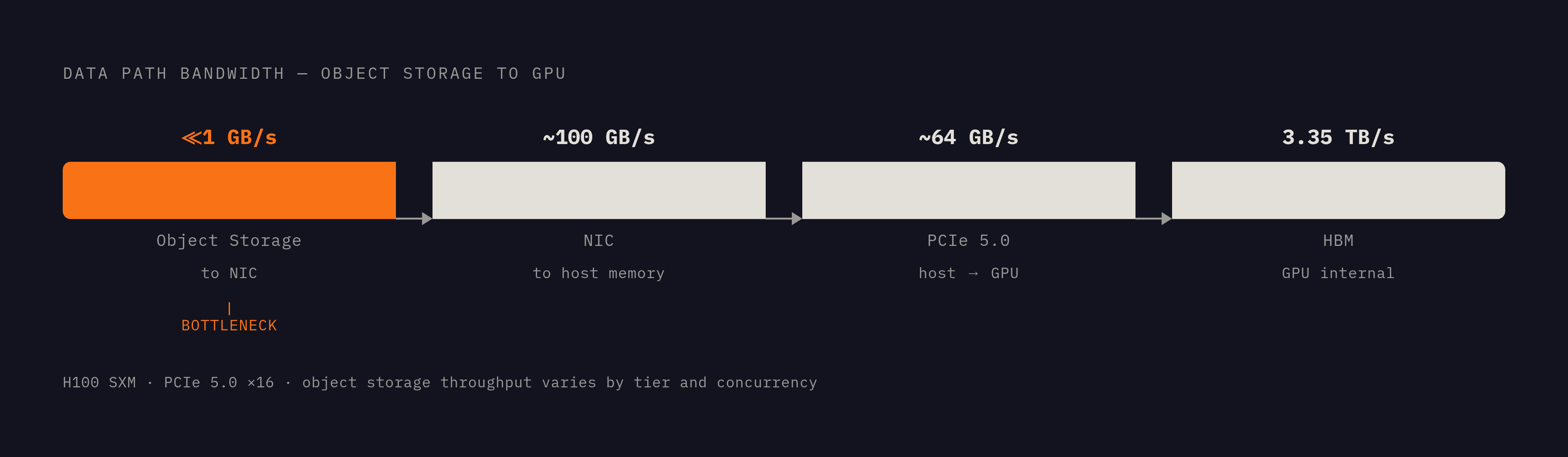
The data path is like a chain of pipes. The narrowest part sets how fast data can flow, even if the rest has room for more. Between object storage and the NIC, throughput depends on the storage tier, concurrent request count, and network path. NIC-to-host-memory bandwidth is typically tens to hundreds of GB/s on a modern server and is rarely the loading constraint.
The next boundary is CPU-to-GPU transfer. PCIe 5.0 provides approximately 64 GB/s, compared with 3.35 TB/s of HBM bandwidth on H100 SXM. HBM governs in-GPU operations. For weight streaming, the speed limit is usually still on the path from object storage to NIC.
This distinction explains why overlap sometimes disappoints. At 500 MB/s over NFS, reads take most of the time, so little time can be saved by hiding transfers behind them. At 3–4 GB/s on local NVMe, overlap saves meaningful time on large models. GPUDirect Storage removes the CPU bounce buffer from the NVMe or network-storage path, but it cannot make up for an upstream source that sends bytes too slowly.
What MLPerf Storage v3.0 benchmarks reveal about storage pipeline performance
MLCommons published MLPerf Storage v3.0 results on September 1, 2026, covering training throughput, checkpointing, and new vector database and KV cache workloads. The release also added an S3 data layer to the existing POSIX layer. About one-sixth of the submissions used S3 access. Object-native pipelines are represented, but they do not dominate the results.
Checkpoint submissions demonstrate the scale of storage throughput. An Everpure FlashBlade//EXA configuration with 30 data nodes reached 877.5 GiB/s of write bandwidth. Azure Managed Lustre reached 642.2 GiB/s from a 4,096 TiB deployment with 128 clients. These results measure checkpoint write bandwidth independently on different configurations.
The benchmark’s scope limits how those figures transfer. It replays configured I/O patterns rather than executing framework code, so it excludes genuine torch.save behavior, FSDP sharded-checkpoint coordination, and checkpoint file-creation metadata storms. Its new KV cache workload nevertheless provides a reproducible comparison of a relevant access pattern. The results establish measurable storage capabilities, while deployment tests must establish application performance.
What storage architecture matters most for reducing LLM inference latency at scale
A streaming loader exposes sustained storage bandwidth. Consistent hashing spreads shards across nodes so that concurrent reader threads do not all converge on one server, as in systems such as NVIDIA AIStore. Erasure coding changes the capacity economics, reducing storage overhead from 2–3× with replication to roughly 1.2–1.5× at similar durability. The trade-off is CPU work on reads.
Hot weight shards sit on local NVMe, warm shards on a shared parallel filesystem, and cold shards in S3-compatible object storage. Streaming gains most when the hot tier holds the most-requested models. This is the connection between NVMe tiering and cost per token, because reducing loading waits can reduce allocated GPU time spent outside serving, although the supplied evidence does not quantify a per-token saving.
Transport and I/O scheduling also shape sustained throughput. DeepSeek 3FS demonstrated lower data-access latency and improved I/O parallelism through RDMA in distributed AI training storage. Most cloud object stores still use TCP-based HTTP, so having an S3 interface alone does not mean there is an RDMA data path. High-concurrency reads and bursty writes also benefit from lower per-I/O overhead through io_uring submission queues. These properties need to be built into the storage design, while vLLM and SGLang can connect to it through configuration changes.
KV cache offloading as the inference-time extension of the same streaming problem
Once weights are in memory, moving KV cache during inference can run into the same transfer limits. This is distinct from decode-phase weight reads within HBM. In long-document Q&A with a short question, tens of gigabytes of cache may cross PCIe, taking far longer than computing the new tokens. A fast storage backend still feeds a much narrower CPU-to-GPU link.
Hot cache stays in VRAM, warm cache in CPU DRAM, cold cache on local NVMe, and shared or persistent cache in network storage. LMCache supports this pattern for vLLM, SGLang, and NVIDIA Dynamo and reports latency reductions of 3–10× on cache-hit-heavy workloads. An 8-GPU inference node can justify 1–2 TB of system memory as a lower-cost extension of VRAM capacity.
Lossless compression can reduce the bytes crossing those boundaries without sacrificing output quality. The evidence must remain specific, however. DFloat11, presented at NeurIPS 2025, compresses BF16 model weights through Huffman coding of exponent bits and decompresses them on the GPU before matrix multiplication. It demonstrates lossless weight compression with bit-for-bit identical outputs. Cache compression and fast storage address complementary constraints, but gains require validation on the actual cache path.
What checkpoint and recovery performance adds to the storage design requirements
A shared AI storage platform must handle writes as well as reads. Modern LLM training checkpoints every 500–2,000 steps, writing hundreds of gigabytes of distributed model state to persistent storage. The common pattern uses parallel filesystems during active training and asynchronously replicates critical checkpoints to S3-compatible storage.
TierCheck, introduced in 2026, separates high-frequency differential checkpoints from low-frequency base checkpoints across local memory, peer memory, and remote persistent storage. ECCheck, presented at ICDCS 2025, applies erasure coding to in-memory checkpoints for distributed DNN training. For a platform serving loading, checkpointing, and recovery, tiering, efficient high-concurrency I/O, and capacity-efficient durability are core requirements rather than optional additions to a read-optimized backend.
Building and validating a weight streaming pipeline: what to instrument and what to avoid
Validation should begin with separate timing for weight transfer and KV cache warmup. Compare loading with and without --load-format runai_streamer on the same hardware, object store, and network path. Then measure warmup across the first N requests separately. It contributes to total time-to-first-token but is not a weight-streaming result.
Concurrency tuning should follow the measured bottleneck. Increase RUNAI_STREAMER_OBJ_CONCURRENCY, or its legacy fallback where applicable, until the NIC is saturated without overloading storage. Use 64 MB upload blocks and a private endpoint, and validate GDS on the NVMe path to remove the CPU bounce buffer. MLPerf’s KV cache and S3 tests provide reproducible backend comparisons, but live framework tests must establish production behavior.
GitHub and community chat platforms offer ways to find benchmark material and get help from the community.
Sources
- The Energy Cost of Execution-Idle in GPU Clusters
- Eliminate LLM Cold starts: Load models up to 6x Faster with Azure Blob Storage and Run:AI Model Streamer - Azure SDK Blog
- DUAL-BLADE: Dual-Path NVMe-Direct KV-Cache Offloading for Edge LLM Inference
- Building py-kvcache: A Performance Characterization of External KV Caching for vLLM with NVMe SSDs