Identifying Storage I/O as the Bottleneck in GPU Utilization Profiles
Storage I/O, not GPU compute, limits inference throughput.
Every serving team has seen the same puzzling dashboard: GPU utilization reads high, and yet throughput stays stubbornly low and latency refuses to improve. The number on the screen is not lying, but it is not measuring what most people assume it measures.
Why GPU utilization numbers mislead: the gap between peak compute and what actually runs
Standard monitoring tools report GPU utilization as a binary question answered over time: was the GPU doing something during this sampling window, or not. A GPU that is stalled, waiting on a memory request that has not yet returned, can still register as busy, because the counter tracks occupancy of the execution pipeline rather than whether that pipeline is advancing useful work. This is the single most visible health metric on most monitoring dashboards, and it cannot tell apart a GPU crunching numbers from a GPU parked in traffic, which matters enormously for anyone provisioning GPU clusters for large language model inference. A team can read a utilization chart that stays consistently high, conclude the hardware is the limiting factor, buy more of it, and watch the new cluster post the same disappointing tokens-per-second numbers, because the constraint was never compute capacity to begin with. Getting past this requires a more precise vocabulary for what a GPU is doing at any given moment, and that vocabulary starts with a different kind of chart entirely.
What the Roofline Model Reveals About Decode
The real performance ceiling during LLM decode is memory bandwidth, not arithmetic throughput: the decode phase of LLM inference sits deep in the memory-bound regime of the roofline model, where the GPU issues reads far faster than any memory tier can satisfy them. Operations with low arithmetic intensity sit on a rising slope where the ceiling is bandwidth; operations with high intensity sit on a flat ceiling where compute is the limit, and the point where the slope meets the flat ceiling is called the ridge point. That is not a rounding error or a tuning problem. The GPU issues read requests for weights and cached state far faster than any tier of memory can return them, so the ceiling that matters during decode is never compute at all.
This gap is not closing on its own. Compute throughput has scaled faster than memory bandwidth across successive GPU generations, which pushes the ridge point higher with each new chip and widens, rather than narrows, the memory-bound territory where decode lives. Every new GPU generation makes the utilization-number illusion described above more severe, not less, because the mismatch between what the chip can compute and what it can be fed keeps growing.
Inference I/O is not one flow but three: model weight I/O, KV cache I/O, and activation I/O, each drawing from a different rung of the memory hierarchy. Fixing one tends to shift pressure onto another. A single optimization rarely holds for long in production. Storage enters this picture the moment HBM cannot hold everything decode needs. A large model already consumes tens of gigabytes in FP16 weights alone, and KV cache under long-context or high-concurrency load overflows HBM into CPU DRAM and then NVMe, stretching the roofline analysis across tiers with wildly different bandwidth and latency. This matters more during decode than at any other stage, because inference runs in two phases with opposite characters: prefill is compute-bound and parallel, while decode is memory-bound and sequential, requiring the full weight set and a growing KV cache to stream through memory before a single token comes out. A stall during decode does not cost one token. It costs every token after it, compounding across the entire response.
Three Bottleneck Signatures in a GPU Profile
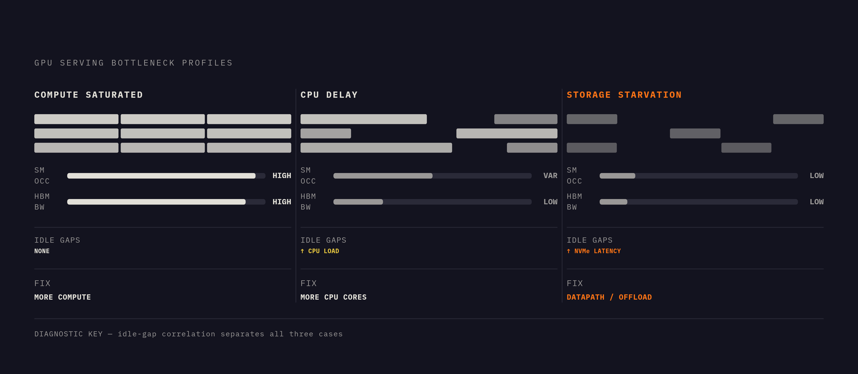
Three distinct problems can produce a low-throughput cluster with a confusing utilization chart: storage I/O starvation, compute saturation, and CPU-side delays. Each leaves its own signature in a profiling trace, and mistaking one for another sends an engineering team chasing the wrong fix.
Compute saturation shows sustained, high SM occupancy across both prefill and decode, with tensor core utilization near its ceiling during prefill. Memory throughput is high as well, the GPU consuming data as fast as it arrives, and this is the one case where adding more compute capacity genuinely helps. Latency breakdowns in this scenario show kernel execution time itself dominating the trace, not idle gaps between kernels.
CPU-side delay looks different and is easy to mistake for a GPU problem. Multi-GPU LLM serving frequently degrades because CPUs cannot keep the GPUs fed, not because the GPUs are saturated: underprovisioned CPU cores delay kernel launches, stall NCCL collectives, and slow tokenization. In a profiling trace this appears as a gap between when one kernel finishes and the next one launches, with the GPU sitting idle while HBM occupancy and IOPS both stay low, the detail that separates it from storage starvation. Agentic and multi-turn workloads amplify this: high prefix-cache reuse reduces GPU-side prefill work while the CPU must still tokenize the full accumulated context at every turn, widening the imbalance. The remedy here is simply more CPU cores, restoring responsiveness without any change to the storage layer.
Storage I/O starvation produces a signature that shows up specifically during decode, not prefill: SM occupancy drops as the GPU finishes a step and then waits, while prefill can look entirely healthy because it is compute-bound and its working set already fits in HBM. During the idle interval, read bandwidth is also low despite there being data still to process, so the pipeline has stalled further upstream, at the DRAM or NVMe tier. These stalls line up in time with spikes in storage latency: any profiling setup that exposes NVMe queue depth or I/O latency alongside the GPU timeline will show the two curves moving together. The IOPS pattern also gives it away. Storage-starved inference shows high-frequency, small, random reads, a fundamentally different demand than the large sequential reads that characterize training workloads.
| Signature | SM occupancy | HBM bandwidth | Idle-gap correlation | Fix | |---|---|---|---|---| | Compute saturation | High, sustained | High | None (kernel time dominates) | More compute | | CPU-side delay | Variable | Low during gaps | Correlated with CPU load, not storage | More CPU cores | | Storage I/O starvation | Low in decode only | Low during idle intervals | Correlated with NVMe latency spikes | Fix datapath or offload strategy |
KV Cache Overflow as the Common Trigger for Storage I/O Starvation
KV cache growth is the single most common reason a serving stack crosses from comfortably HBM-resident operation into storage-bound territory. At long context lengths and high concurrency, KV cache routinely exceeds the memory footprint of the model weights themselves, and the overflow lands on NVMe at the point in the pipeline where it hurts most: mid-decode. The scale involved is not marginal. Serving a large model with an FP16 KV cache at a context length of one million tokens demands memory beyond what a single 80 GB GPU can hold, which makes offloading to another tier an architectural inevitability at long context rather than a rare edge case.
Even before offloading becomes necessary, a substantial amount of HBM is wasted through fragmentation. Traditional inference systems allocate KV cache in contiguous blocks, and a large share of that allocated memory sits unused, reserved but not doing any useful work. PagedAttention addresses this directly by managing KV cache in non-contiguous pages, cutting waste sharply and allowing higher effective batch sizes within the same HBM budget. That technique buys more room, but it does not repeal the underlying physics: once HBM genuinely fills, pages must be evicted, and the I/O path to CPU DRAM or NVMe becomes the new bottleneck.
This is where the profiling signature from the previous section comes from. When a KV page gets evicted mid-sequence, the decode step that needs it stalls until it can be read back, producing the low-SM-occupancy idle interval with correlated storage latency described above. The eviction event is the mechanism, and the idle gap on the GPU timeline is its visible trace.
How the storage datapath itself amplifies or masks the bottleneck depending on which I/O stack you run
The same physical NVMe device can deliver very different effective bandwidth depending on the software sitting between it and the GPU. Overhead in the conventional Linux I/O path inflates tail latency and hides how much the device could actually deliver. That conventional path runs requests through system calls, interrupt handling, kernel queues, and redundant memory copies, and prior studies of training workloads report that a substantial share of end-to-end training time, ranging from roughly a tenth to more than two-thirds, is lost to I/O stalls while GPUs wait for the software stack to finish processing requests.
The right datapath depends on the phase of work. For inference, dominated by small, random reads, io_uring delivers the lowest latency with competitive IOPS for that access pattern, while SPDK is limited to raw block devices without POSIX file-system support, which narrows where it can be applied for this kind of workload. For pre-training and fine-tuning, dominated by large sequential reads and writes, GPUDirect Storage cuts load times and host CPU usage by moving data directly between NVMe and GPU memory over DMA, bypassing host DRAM entirely.
The wall-clock difference is not subtle. On an H100 SXM5 with a single Gen4 NVMe drive, a checkpoint that runs through the conventional path takes many times longer than the same checkpoint run with GDS. Scaled up to an 8×H200 SXM5 node with four Gen5 NVMe drives, the checkpoint completes in roughly 8 seconds with GDS, a fraction of the time the conventional path requires. Those seconds are the datapath choice made visible in a number every practitioner recognizes instantly.
Kernel-bypass and zero-copy transfer, moving data straight from storage into GPU memory, cannot coexist with traditional file-based I/O built on system calls and buffered copies. A team running legacy NFS or slow object storage under an inference workload is not simply leaving performance on the table relative to NVMe. The architecture itself cannot serve that access pattern at any speed. At networked scale, the same principle holds: coupling fast NVMe media with an RDMA transport and GPU-aware data movement can deliver 4 TB/s aggregate throughput to a system the size of NVIDIA's Eos AI supercomputer, showing what an end-to-end datapath designed for AI workloads is capable of.
Reading the Profile in Practice
Diagnosing storage I/O starvation with any confidence means watching two layers of the stack at once: GPU-side signals (SM occupancy, kernel launch gaps, HBM read bandwidth over time) and storage-side signals (NVMe queue depth, I/O latency distribution, IOPS rate and request size). Neither layer alone gives an answer that rules out the other explanations covered above.
On the GPU side, NVIDIA Nsight Systems renders a timeline where kernel launch gaps appear as literal white space between colored kernel bars. The width and placement of that white space relative to decode steps is the first thing worth reading in the trace. Comparing SM occupancy during decode kernels, identifiable by their sequential, single-token pattern, against SM occupancy during prefill is the next step: a wide gap, healthy during prefill and collapsed during decode, points to memory or I/O starvation rather than compute saturation. The HBM bandwidth counters settle the question further. If HBM read bandwidth is also low during that idle interval, the stall sits upstream of HBM itself, meaning data is not arriving from CPU DRAM or NVMe fast enough to fill HBM, let alone keep the compute units busy.
On the storage side, NVMe queue depth over time separates a healthy, I/O-bound system from a starved one. A healthy system shows sustained queue depth, while a storage-starved GPU system shows depth spiking and then draining as the GPU catches up on a backlog, and that drain lines up with the idle interval already visible in the GPU timeline. Request size distribution confirms the diagnosis: inference generates many small, random reads against individual KV pages or weight shards, while training generates large sequential reads, and finding the former on a system tuned for the latter confirms an architectural mismatch. Average throughput is the wrong number to anchor on here. Tail latency at p99 matters more for inference, because a single slow read on one KV page blocks the decode step waiting on it and adds its full latency directly to that token's generation time.
CPU-side instrumentation serves as the ruling-out step that closes the loop. Kernel launch latency histograms in Nsight separate CPU-induced gaps, which vary with CPU load and show no relationship to storage queue depth, from storage-induced gaps, which correlate with NVMe latency spikes. CPU-starved configurations show kernel launch latency inflated from microseconds into milliseconds, a shift easily visible in the profiler histogram and impossible to confuse with a storage stall once both traces sit side by side.
Lossless Compression and Quantization Change the I/O Budget
Everything above describes how to locate a storage bottleneck once it exists. The other lever available to a serving team is reducing how much data has to move through that bottleneck. Model weights and KV cache entries are both compressible, and lower-precision formats such as quantized weights and reduced-precision KV cache representations shrink the volume of bytes that must travel from NVMe through DRAM into HBM on every decode step. A smaller weight footprint means less has to stream per step during the memory-bound decode phase described in the roofline section above, and a smaller KV cache footprint means more of the working set can stay resident in HBM before eviction to CPU DRAM or NVMe becomes necessary, directly reducing how often the eviction-driven idle interval described earlier occurs. Format and precision choices set the size of the I/O problem before any storage engineering enters the picture; a datapath tuned with io_uring or GDS moves whatever bytes it is handed efficiently, but the number of bytes handed to it is decided earlier, in how the model and its cache are represented. Treating compression and quantization as part of the I/O budget, not as a separate accuracy-versus-speed tradeoff, keeps the storage tier from having to compensate for data volume decisions made upstream of it.